Formal semantics
Readings
- Pre-recorded lecture: Operational semantics
- Pre-recorded lecture: Lambda calculus
- Operational semantics, Sections Seções 8.5 (you can ignore “completeness and consistency”) and 8.6.
Introduction to Programming Languages, entry on semantics.
- The lambda calculus, Sections 5.1, 5.2 (pag. 139 to 159).
Recommended readings
- Semantics with applications: an appetizer, Chapters 1 and 2.
- A bit on the history of computing, Chapters 1-3.
- A Minimalistic Verified Bootstrapped Compiler: A recent paper on writing a simple compiler with a full formal semantics that is verified correct, i.e., proves that the x86 assembly code it produces is equivalent to the original code.
Overview
Syntax defines what the programs we write look like, while semantics defines their meaning.
The semantics of a language
L1can be defined via a interpreted forL1in another languageL2with a well-defined semantics.Note this is the approach we’ve taken with our expression language, using SML as the interpreter language.
However, how do we define the semantics of
L2?
- There are formal notations to define the semantics of programming languages. A common way is with operational semantics:
- Specifies, step by step, what happens while a program is executed.
- Writing on the board (in recording) for operational semantics
- Writing on the board (in recording) for lambda calculus
Operational semantics
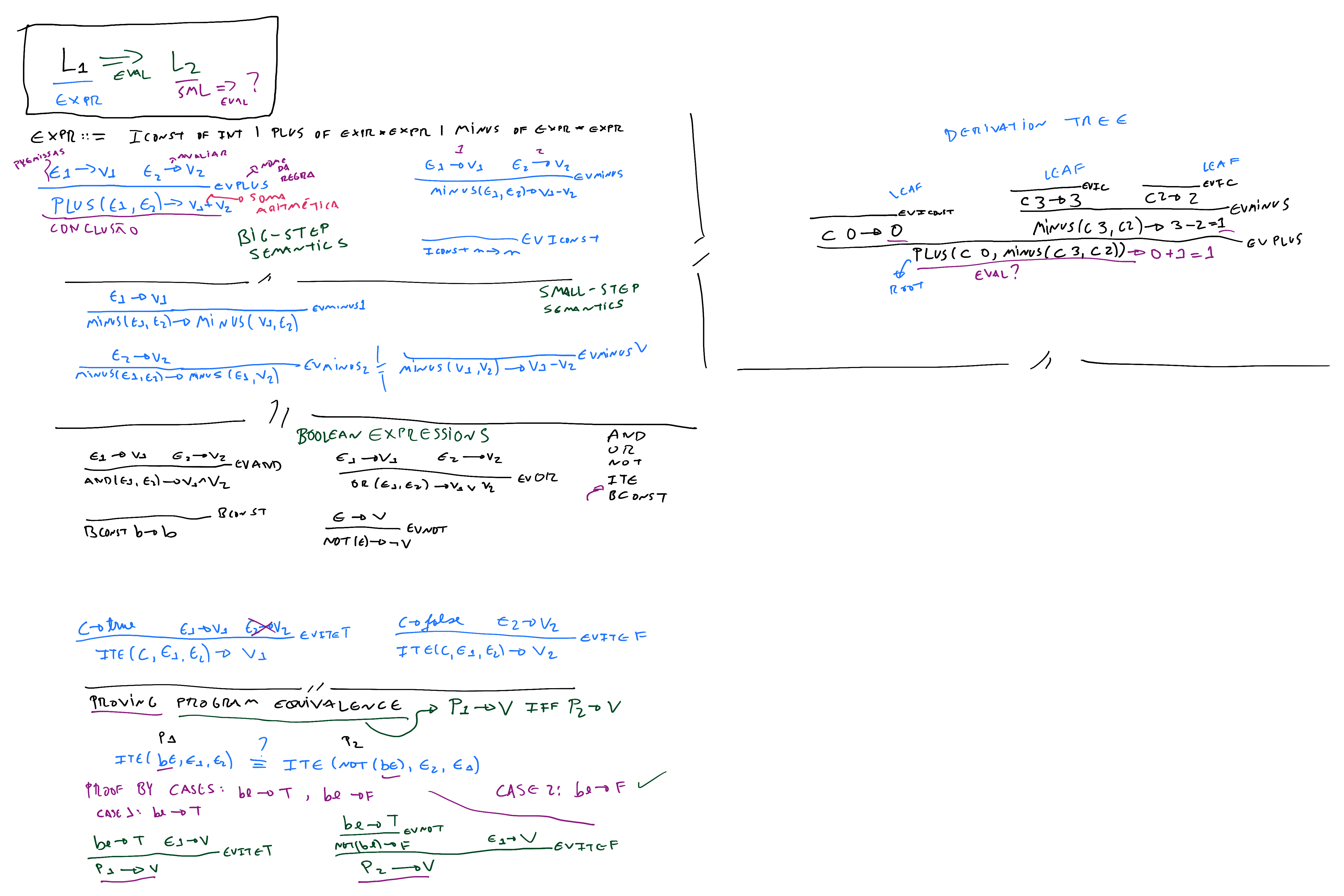
The specification of an execution is step is given by inference rules
- Judgements for writing inference rules:
- Premises are written above the line.
- Conclusion below the line.
- Label by the lines denote the rule name
- Arrows represent how expressions are evaluated.
- Considering the expressions in the basic version of our previously defined language, their semantics is:
 E1 -> v1      E2 -> v2              E1 -> v1      E2 -> v2
------------------------ EvPlus     -------------------------- EvMinus
Plus(E1, E2) -> v1 + v2             Minus(E1, E2) -> v1 - v2

------------- EvIConst
IConst n -> n
- The above establishes how expressions built with
IConst,PlusandMinusare evaluated, i.e., in terms of the semantics of the arithmetic functions+,-.- Note this is not dependent on a programming language but on arithmetic itself.
Big step and small step semantics
- The above is often called “big step semantics” (also “natural semantics”)
- There is also “small step semantics”, in which a rule does only one computation (“one step”) at a time:
          E1 -> E1'                             E1 -> E1'
-----------------------------EvPlus1      ---------------------------------EvMinus1
Plus(E1, E2) -> Plus(E1', E2)             Minus(E1, E2) -> Minus(E1', E2)

          E2 -> E2'                             E2 -> E2'
-----------------------------EvPlus2      ---------------------------------EvMinus2
Plus(E1, E2) -> Plus(E1, E2')             Minus(E1, E2) -> Minus(E1, E2')


---------------EvIConst
IConst n -> n

-----------------------EvPlusV   -------------------------EvMinusV
Plus(v1, v2) -> v1 + v2           Minus(v1, v2) -> v1 - v2
How to define the semantics of Ite?
- Let’s go back to use big step semantics.
- Since
Iterelies on Boolean expressions, we must define their semantics as well.
 E1 -> v1      E2 -> v2              E1 -> v1      E2 -> v2
------------------------EvAnd     --------------------------EvMinus
And(E1, E2) -> v1 ∧ v2               Or(E1, E2) -> v1 v v2

                                    E -> v
-------------EvBConst             ---------------EvNot
BConst n -> n                       Not(E) -> ¬v1
- Now we can define the rules for
IteE1 -> true E2 -> v2 E1 -> false E3 -> v3 -------------------------EvIteT or --------------------------EvIteF Ite(E1, E2, E3) -> v2 Ite(E1, E2, E3) -> v3
Note that the above rules rely on Boolean logic itself.
Evaluation as derivation trees
- Evaluating an expression corresponds to bulding a derivation tree
- the root of the tree is the evaluation of the original expression
- the premises must be roots of subtrees justifying their evaluations and so on
- The derivation tree below corresponds to the evaluotion of
Plus(IConst 0, Minus(IConst 3, IConst 2))
                       -------------EvIConst  -------------EvIConst
                       IConst 3 -> 3          IConst 2 -> 2
-------------EvIConst  --------------------------------------EvMinus
IConst 0 -> 0          Minus(IConst 3, IConst 2) -> 3 - 2 = 1
--------------------------------------------------------------EvPlus
  Plus(IConst 0, Minus(IConst 3, IConst 2)) -> 0 + 1 = 1
Static vs dynamic semantics
- Static semantics: program meaning known at compilation time.
- Type errors
- Use of undefined variables
- Dynamic semantics: program meaning known at run time
- Memory management errors can be very hard to detect statically.
Program equivalence
- With a formal semantics we can reason statically about programs
- We can for example possibly prove that two programs are equivalent
- To say that two programs
P1andP2are equivalent:P1 -> v iff P2 -> vi.e., they produce the same value when they produce some value. Such proofs can be done in general via induction on the derivation trees that can be built with the inference rules used to evaluate the expression.
- To say that two programs
- Let’s consider the following program equivalence problem, for programs in our expression language with the above semantics. Prove that
Ite(c,e1,e2) = Ite(Not(c),e2,e1)
for any expression c, e1, e2 (of the correct types for the constructor Ite).
- Since
cis a Boolean expression, it can be evaluated either totrueor tofalse. We consider each case:Case 1:
c -> trueThe derivation of
P1will be:... ... --------- -------- c -> true e1 -> v ------------------------EvIteT Ite(c, e1, e2) -> vSince
c -> true, we know that... --------- c -> true ----------------EvNot Not(c) -> false
thus the derivation of P2 will be
...
---------
c -> true                  ....
----------------EvNot    --------
Not(c) -> false           e1 -> v
----------------------------------EvIteF
  Ite(Not(c), e2, e1) -> v
- Case 2:
c -> falseTry it yourself. :)
Solution
The derivation of P1 will be:
...            ...
---------      --------
c -> false      e2 -> v
------------------------EvIteF
  Ite(c, e1, e2) -> v
Since c -> false, we know that
...
---------
c -> false
----------------EvNot
Not(c) -> false
thus the derivation of P2 will be
...
---------
c -> false                  ....
----------------EvNot    --------
Not(c) -> true           e2 -> v
----------------------------------EvIteT
  Ite(Not(c), e2, e1) -> v
- In all generality one needs to consider as well the non-terminating executions:
P1 -> stuck iff P2 -> stuckfor some notion of “stuck”.
Program equivalence as SMT
SMT and cvc5
Satisfiability Modulo Theories (SMT) is the satisfiability problem in first-order logic modulo a set of background theories. Thus one asks whether a given formula is satisfiable according to a fixed interpretation of some symbols (for example that the symbol + in a formula refers to arithmetic addition).
The cvc5 SMT solver is a state-of-the-art solver for SMT problems. It can attempt to solve any problem formulated in SMT. The system accepts SMT-LIB as an input format as well as multiple APIs (in Python, C++, and Java).
Program equivalence
To install cvc5 and use it in Python you can do (with an up to date Python installation):
pip install cvc5
To check in SMT the equivalence of two programs we need to encode the language of these programs into the SMT language. SMT solvers have builtin support for Boolean and Integer arithmetic, as well as if-then-else and variable assignment. Therefore we can directly encode our expression language into it.
Given our equivalence problem
Ite(c,e1,e2) = Ite(Not(c),e2,e1)
we need to first introduce variables to represent c, e1 and e2. Since the first is a Boolean and the last two are integers, we use the respective builtin types in cvc5:
c = Bool('c')
e1, e2 = Ints('e1 e2')
Next we create the programs which we want to test the equivalence to, using the cvc5 builtin operator for if-then-else (If) and the bultin operator for Boolean negation (Not):
p0 = If(c, e1, e2)
p1 = If(Not(c), e2, e1)
Finally we can ask the solver p0 and p1 are equivalent. For them to be equivalent it must be the case that for every value of c, e1 and e2, it is true that p0 and p1 are equal. This means that it is valid that p0 and p1 are equal.
There is a duality between validity (a statement is always true) and satisfiability (a statement can be true). That is that a formula φ is valid if and only if ¬φ is unsatisfiable, i.e., a formula is always true if it cannot be the case that its negation can be true.
Since an SMT solver answers satisfiability queries, the equivalence of p0 and p1, which requires the validity that they are equal, is phrased as the satisfiability problem of whether they are disequal. If that is unsatisfiable, then p0 and p1 are equivalent.
The cvc5 python API provides a solve command that accepts satisfiability queries:
solve(p0 != p1)
The answer will be “no solution”, which says that the query is unsatisfiable.
The complete python program is:
from cvc5.pythonic import *

if __name__ == '__main__':
    c = Bool('c')
    e1, e2 = Ints('e1 e2')

    p0 = If(c, e1, e2)
    p1 = If(Not(c), e2, e1)

    solve(p0 != p1)
The above formulation can be written as well in SMT-LIB, with the following syntax:
(set-logic QF_UFLIA)

(declare-const c Bool)
(declare-const e1 Int)
(declare-const e2 Int)

(define-fun p0 () Int (ite c e1 e2))
(define-fun p1 () Int (ite (not c) e2 e1))

(assert (not (= p0 p1)))

(check-sat)
A file with the above content can be passed to a binary of cvc5 (downloads available here), which will yield the answer unsat to symbolize that it is an unsatisfiable problem.
The Lambda Calculus
The lambda calculus is a notation to describe computations
- It offers a precise formal semantics for programming languages.
The Church-Turing thesis:
The lambda calculus is as powerful as Turing machines.
In other words, these are equivalent models of computation, i.e., of defining algorithms.
- Turing and Church indepedently proved, in 1936, that:
- program termination is undecidable (with Turing machines)
- program equivalence is undecidable (with lambda calculus)
- Thus both showed that the Entscheidungsproblem, to David Hilbert’s dismay, is unsolvable.
- There are undecidable problems. There are problems which we cannot solve, for every instance of the problem, with algorithms.
- Both built on Kurt Gödel’s incompleteness theorems, which first showed the limits of mathematical logic.
Notation
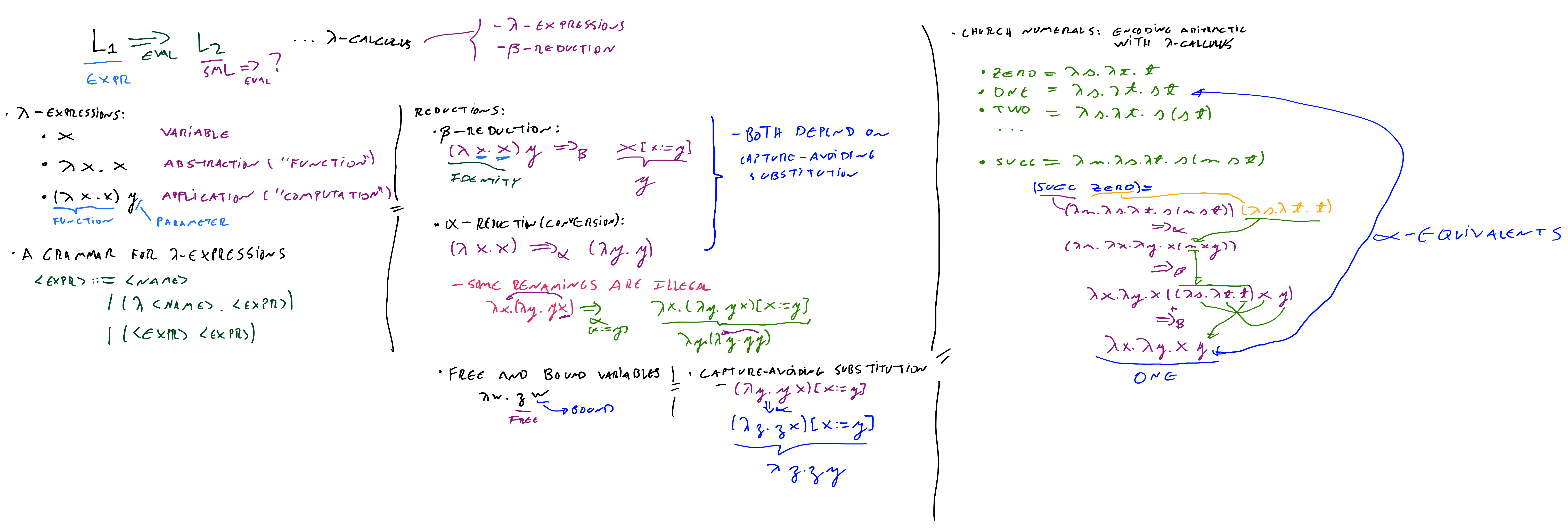
The lambda calculus consists of writing λ-expressions and reducing them. Intuitively it is a notation for writing functions and their applications.
A λ-expression is either:
- a variable
x - an abstraction (“a function”)
λx . xin which the variable after the lambda is called its bound variable and the expression after the dot its body.
- an application (“of a function to an argument”)
(λx . x) z
in which the right term is the argument of the application. When written without parenthesis assume left-associativity.
This means that λ-expressions follow the syntax:
<expr> ::= <name>
         | (\lambda <name> . <expr>)
         | (<expr> <expr>)
Expressions can be manipulated via reductions. Intuitively they correspond to computing with functions.
Beta (β-reduction)
- Captures the idea of function application.
- It is defined via substitution:
- an application is β-reduced via the replacement, in the body of the abstraction, of all occurrences of the bound variable by the argument of the application.
- Consider the example application above:
(λx . x) z
=>_β
z
Intuitively (λx . x) corresponds to the identity function: whatever expression it is applied to will be the result of the application.
Alpha (α-conversion)
- Renames bound variables.
(λx . x) =>_α (λy . y) - Expressions that are only different in the names of their bound variables are called α-equivalent.
- Intuitevely, the names of the bound variables do not change the meaning of the function.
- For example, both
(λx . x)and(λy . y)correspond to the identity function.
Free and bound variables
- Not all renaming is legal.
(λx . (λy . y x)) =>_α (λy . (λy . y y)) - This renaming changes what the function computes, as
xwas renamed to a variable,y, that was not free in the body of the expression.- As an example, consider the following SML code:
val y = 1
fun f1 x = y + x
fun f2 z = y + z
fun f3 y = y + y
You will note that
f1andf2are equivalent, whilef1andf3are not. - Free variables are those that are not bound by any lambda prefix enclosing it.
(λw . z w)- In the body of the expression
wis bound whilezis free.
- In the body of the expression
Capture-avoiding substitutions
- To avoid the above issue, α-conversion must be applied with capture-avoiding substitutions:
- When recursively traversing the expression to apply the substitution, if the range of the substitution contains a variable that is bound in an abstraction, rename the bound variable so that the free variable is not captured.
- In the above example, to do a substitution of
xbyyon(λ x . (λ y . y x)), written(λx . (λy . y x))[x:=y]
we will do
(λ y . y x)[x:=y]. Sinceyis bound in the expression in which we are doing the substitution, we rename the bound variable to avoid capture:(λy . y x) =>_α (λz . z x)Now we can do
(λz . z x)[x:= y]so that the variablex, which is free in this expression, remains so after substitution. Thus we obtain:(λx . (λy . y x)) =>_α (λy . (λz . z y))which are equivalent functions.
- The same principle applies to β-reduction: it is applied with capture-avoiding substitutions to avoid issues with capture.
Encodings
- With λ-expressions and β-reduction we can do all computation. Every algorithm that exists.
- The caveat: you must first encode in λ-expressions whatever you mean.
Numbers (Church numerals)
- Encodings are about conventions. We agree on the meaning of something and build accordingly.
- A number is a function that takes a function
splus a constantz. The numberNcorresponds toNapplications ofstoz.
Zero  = λs. λz. z
One   = λs. λz. s z
Two   = λs. λz. s (s z)
Three = λs. λz. s (s (s z))
...
The successor function
SUCC = λn. λy. λx. y (n y x)
- If we apply the successor function to
Zerowe must obtainOne:SUCC Zero = (λn.λy.λx.y(nyx))(λs.λz.z) =>_β λy.λx.y((λs.λz.z)yx) =>_β λy.λx.yx = One - Similarly, we should obtain that
SUCC One = TwoSUCC One = (λn.λy.λx.y(nyx))(λs.λz.sz) =>_β λy.λx.y((λs.λz.sz)yx) =>_β λy.λx.y(yx) = TwoAnd so on. One can prove via induction that
Succ Nis always equal to the corresponding natural number ofNplus one.
Addition
ADD = λm.λn.λx.λy.m x (n x y)
- Again we can see the expected behavior with examples:
ADD Two Three = (λm.λn.λx.λy.m x (n x y)) Two Three =>_β λx.λy.Two x (Three x y) =>_β λx.λy.Two x (x (x (x y))) =>_β λx.λy.(λs.λz.s (s z)) x (x (x (x y))) =>_β λx.λy.x (x (x (x (x y)))) = Five - Note that addition can be defined in terms of the successor function
- Summing
nwithmcorresponds to applying the successor functionntimes tom.- Our number encoding is precisely “number
Nis applying functionsto constantzNtimes”, i.e.,ADD = λm. λn. m SUCC n
- Our number encoding is precisely “number
- Rephrasing the above example:
ADD Two Three =
 Two SUCC Three =
(λs.λz.s (s z)) SUCC Three =>_β
(λz. SUCC (SUCC z)) Three =>_β
SUCC (SUCC Three) =>_β
SUCC Four =>_β
Five
The above is enough to encode Presburger arithmetic .
- One can encode anything we are used to do with computers.
Note that all complexity lies in how to encode. Once the encoding is done, computation is merely doing β-reduction.
Boolean algebra (Church Booleans)
T  = λx.λy.x
F = λx.λy.y
AND   = λx.λy.xyF
OR    = λx.λy.xTy
NOT   = λx.xFT
- Try it yourself
AND T F = ?
Solution
AND T F =
(λx.λy.xyF) T F =>_β
T F F =
(λx.λy.x) F F =>_β F
OR F T = ?
Solution
OR F T
(λx.λy.xTy) F T =>_β
F T T =
(λx.λy.y) T T =>_β T
NOT T = ?
Solution
NOT T
(λx.xFT) T =>_β
T F T =
(λx.λy.x) F T =>_β F